Algorithm Time Complexity
1. 介绍 (Introduction)
什么是时间复杂度? (What is Time Complexity?)
时间复杂度是衡量算法运行时间与输入规模之间关系的一个指标。它通常使用大O符号来表示。时间复杂度告诉我们算法在最坏情况下的表现。
Time complexity is a measure of the relationship between the running time of an algorithm and the size of its input. It is usually represented using Big O notation. Time complexity indicates the performance of an algorithm in the worst-case scenario.
常见的时间复杂度 (Common Time Complexities)
常见的时间复杂度包括:
- 常数时间复杂度:(O(1)) (Constant Time Complexity)
- 线性时间复杂度:(O(n)) (Linear Time Complexity)
- 对数时间复杂度:(O(\log n)) (Logarithmic Time Complexity)
- 线性对数时间复杂度:(O(n \log n)) (Linear Logarithmic Time Complexity)
- 二次时间复杂度:(O(n^2)) (Quadratic Time Complexity)
- 指数时间复杂度:(O(2^n)) (Exponential Time Complexity)
- 阶乘时间复杂度:(O(n!)) (Factorial Time Complexity)
2. 常数时间复杂度 (O(1)) (Constant Time Complexity)
定义 (Definition)
常数时间复杂度表示算法的运行时间不随输入规模的变化而变化。
Constant time complexity indicates that the running time of an algorithm does not change with the size of the input.
示例 (Example)
访问数组中的某个元素: Accessing an element in an array:
def get_element(arr, index):
    return arr[index]
应用 (Applications)
- 哈希表的查找、插入和删除操作(在理想情况下)。
- Lookup, insertion, and deletion operations in a hash table (in ideal conditions).
3. 线性时间复杂度 (O(n)) (Linear Time Complexity)
定义 (Definition)
线性时间复杂度表示算法的运行时间与输入规模成正比。
Linear time complexity indicates that the running time of an algorithm is directly proportional to the size of the input.
示例 (Example)
计算数组中所有元素的和: Calculating the sum of all elements in an array:
def sum_array(arr):
    total = 0
    for num in arr:
        total += num
    return total
应用 (Applications)
- 遍历数组或链表。
- Traversing an array or a linked list.
4. 对数时间复杂度 (O(\log n)) (Logarithmic Time Complexity)
定义 (Definition)
对数时间复杂度表示算法的运行时间与输入规模的对数成正比。常见于分治算法。
Logarithmic time complexity indicates that the running time of an algorithm is proportional to the logarithm of the size of the input. It is common in divide-and-conquer algorithms.
示例 (Example)
二分查找: Binary search:
def binary_search(arr, target):
    left, right = 0, len(arr) - 1
    while left <= right:
        mid = (left + right) // 2
        if arr[mid] == target:
            return mid
        elif arr[mid] < target:
            left = mid + 1
        else:
            right = mid - 1
    return -1
应用 (Applications)
- 二分查找。
- Binary search.
- 平衡二叉搜索树的操作(如AVL树、红黑树)。
- Operations in balanced binary search trees (e.g., AVL trees, Red-Black trees).
5. 线性对数时间复杂度 (O(n \log n)) (Linear Logarithmic Time Complexity)
定义 (Definition)
线性对数时间复杂度表示算法的运行时间与输入规模和其对数的乘积成正比。
Linear logarithmic time complexity indicates that the running time of an algorithm is proportional to the product of the size of the input and its logarithm.
示例 (Example)
合并排序: Merge sort:
def merge_sort(arr):
    if len(arr) <= 1:
        return arr
    mid = len(arr) // 2
    left = merge_sort(arr[:mid])
    right = merge_sort(arr[mid:])
    return merge(left, right)

def merge(left, right):
    result = []
    i = j = 0
    while i < len(left) and j < len(right):
        if left[i] < right[j]:
            result.append(left[i])
            i += 1
        else:
            result.append(right[j])
            j += 1
    result.extend(left[i:])
    result.extend(right[j:])
    return result
应用 (Applications)
- 合并排序。
- Merge sort.
- 快速排序(平均情况下)。
- Quick sort (average case).
6. 二次时间复杂度 (O(n^2)) (Quadratic Time Complexity)
定义 (Definition)
二次时间复杂度表示算法的运行时间与输入规模的平方成正比。
Quadratic time complexity indicates that the running time of an algorithm is proportional to the square of the size of the input.
示例 (Example)
冒泡排序: Bubble sort:
def bubble_sort(arr):
    n = len(arr)
    for i in range(n):
        for j in range(0, n-i-1):
            if arr[j] > arr[j+1]:
                arr[j], arr[j+1] = arr[j+1], arr[j]
    return arr
应用 (Applications)
- 冒泡排序。
- Bubble sort.
- 选择排序。
- Selection sort.
- 插入排序。
- Insertion sort.
7. 指数时间复杂度 (O(2^n)) (Exponential Time Complexity)
定义 (Definition)
指数时间复杂度表示算法的运行时间与输入规模的指数成正比。
Exponential time complexity indicates that the running time of an algorithm is proportional to an exponential function of the size of the input.
示例 (Example)
计算斐波那契数列(递归): Calculating the Fibonacci sequence (recursively):
def fibonacci(n):
    if n <= 1:
        return n
    return fibonacci(n-1) + fibonacci(n-2)
应用 (Applications)
- 解决NP完全问题(如旅行商问题)。
- Solving NP-complete problems (e.g., the Traveling Salesman Problem).
- 某些递归算法。
- Certain recursive algorithms.
8. 阶乘时间复杂度 (O(n!)) (Factorial Time Complexity)
定义 (Definition)
阶乘时间复杂度表示算法的运行时间与输入规模的阶乘成正比。
Factorial time complexity indicates that the running time of an algorithm is proportional to the factorial of the size of the input.
示例 (Example)
计算所有可能的排列: Calculating all possible permutations:
def permutations(arr):
    if len(arr) == 0:
        return [[]]
    result = []
    for i, num in enumerate(arr):
        for perm in permutations(arr[:i] + arr[i+1:]):
            result.append([num] + perm)
    return result
应用 (Applications)
- 全排列问题。
- Permutation problems.
结论 (Conclusion)
理解不同的时间复杂度及其应用场景对于算法设计和优化至关重要。不同的时间复杂度反映了算法在处理不同规模输入时的效率,选择合适的算法可以显著提高程序的性能。
Understanding different time complexities and their applications is crucial for algorithm design and optimization. Different time complexities reflect the efficiency of an algorithm in handling inputs of varying sizes, and choosing the right algorithm can significantly improve the performance of a program.
时间复杂度可视化代码 (Time Complexity Visualization Code)
为了更直观地理解这些时间复杂度,我们可以用Python绘制出它们的增长曲线。以下是一个示例代码:
# Aemon Wang
# aemooooon@gmail.com

import numpy as np
import matplotlib.pyplot as plt
import math

# 定义输入规模 (Define input sizes)
n = np.linspace(1, 10, 400)
n_factorial = np.arange(1, 10)

# 定义各种时间复杂度函数 (Define different time complexity functions)
complexities = {
    "O(1)": np.ones_like(n),
    "O(log n)": np.log(n),
    "O(n)": n,
    "O(n log n)": n * np.log(n),
    "O(n^2)": n**2,
    "O(2^n)": 2**n,
    "O(n!)": [math.factorial(i) for i in n_factorial],
}

# 绘制图形 (Plot the graph)
plt.figure(figsize=(12, 8))
for label, y in complexities.items():
    if label == "O(n!)":
        plt.plot(n_factorial, y, label=label)
    else:
        plt.plot(n, y, label=label)

plt.ylim(1, 10**5)
plt.xlim(1, 10)
plt.yscale("log")
plt.xlabel("Input Size (n)")
plt.ylabel("Operations")
plt.title("Time Complexity of Different Algorithms")
plt.legend()
plt.grid(True)
plt.show()
结果 (Result)
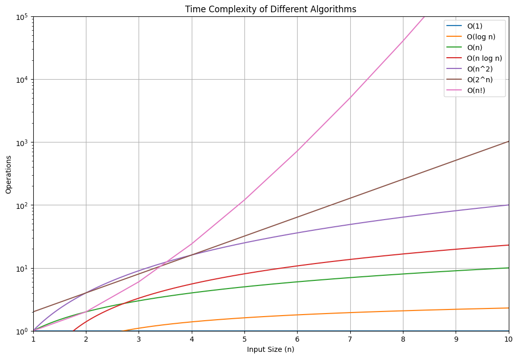
该图展示了不同时间复杂度函数的增长曲线,使用对数坐标轴使得这些复杂度的差异更加明显。通过这些曲线,你可以直观地看到不同算法在处理不同规模输入时的效率差异。
This chart shows the growth curves of different time complexity functions, using a logarithmic scale to make the differences more apparent. By looking at these curves, you can visually understand the efficiency differences of various algorithms when handling inputs of different sizes.
具体解释 (Detailed Explanation)
-
(O(1)): 常数时间复杂度,表示算法的运行时间不随输入规模变化。在图中是一条水平线。
Constant time complexity, indicated by a horizontal line in the chart, means the algorithm’s running time does not change with the size of the input.
-
(O(\log n)): 对数时间复杂度,表示算法的运行时间随输入规模的对数增长。常见于分治算法,如二分查找。
Logarithmic time complexity, shown as a curve that slowly increases, indicates the algorithm’s running time grows with the logarithm of the input size. Common in divide-and-conquer algorithms like binary search.
-
(O(n)): 线性时间复杂度,表示算法的运行时间与输入规模成正比。在图中是一条倾斜的直线。
Linear time complexity, represented by a straight line, means the running time is directly proportional to the size of the input.
-
(O(n \log n)): 线性对数时间复杂度,表示算法的运行时间与输入规模及其对数的乘积成正比。常见于排序算法,如合并排序。
Linear logarithmic time complexity, shown as a curve that rises faster than linear but slower than quadratic, indicates the running time is proportional to the product of the input size and its logarithm. Common in sorting algorithms like merge sort.
-
(O(n^2)): 二次时间复杂度,表示算法的运行时间与输入规模的平方成正比。在图中是一条较陡的曲线。
Quadratic time complexity, represented by a steeper curve, means the running time is proportional to the square of the input size.
-
(O(2^n)): 指数时间复杂度,表示算法的运行时间随输入规模的指数增长。在图中是一条快速上升的曲线。
Exponential time complexity, shown as a rapidly rising curve, indicates the running time grows exponentially with the input size.
-
(O(n!)): 阶乘时间复杂度,表示算法的运行时间随输入规模的阶乘增长。在图中是一条非常陡峭的曲线。
Factorial time complexity, represented by an extremely steep curve, means the running time grows factorially with the input size.